Whiten out variance of the gradients
Curvature is only part of the story. Even on the simplest quadratic, gradient noise can send stochastic gradient descent in the wrong direction.
This post is based on our paper, Stochastic optimization methods through statistical whitening.
Consider an objective function that is a perfectly round bowl, but the gradient is corrupted by noise:
The noise has mean zero and covariance . The Hessian is the identity, so the function is perfectly well conditioned. But the gradient has a thousand times more variance in its second coordinate than in its first. SGD spends much of its effort bouncing along that noisy direction.
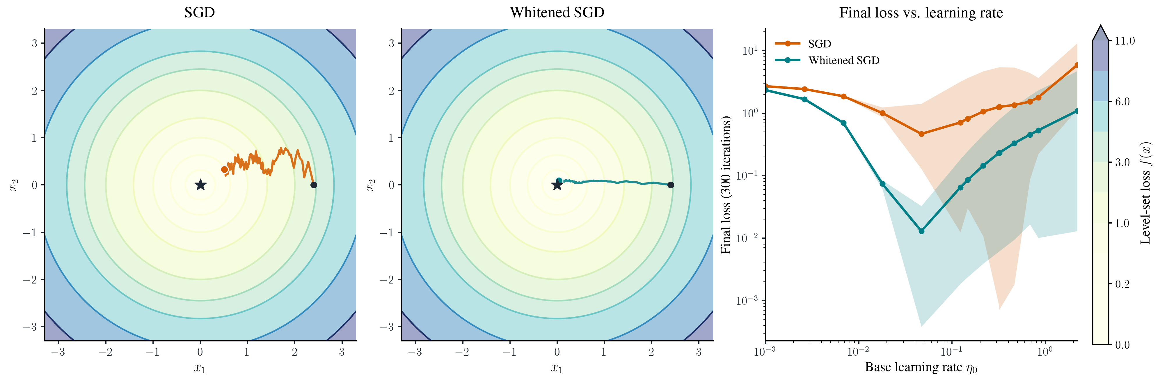
A small learning rate quiets the noise, but also slows progress toward the minimum. Can we treat the two directions differently? The main idea is that we should take cautious and small steps in the direction of low variance, and larger steps in the direction of high variance. We will call this ``whitening the gradient''. Here is a small experiment to illustrate how SGD compares to whitened SGD.
Same bowl. Different noise.
300 steps · paired noise drawsCircles mark the start and endpoints and the cross marks the minimum. The trajectories compare SGD on (1) with the whitened SGD update (2). Both methods use schedule ηₜ = η₀ / √(t + 1).
SGD
Whitened SGD
Loss over iterations
Numerical results
| Method | Loss at selected rate | Best swept rate | Loss at best rate |
|---|
Loading the interactive experiment. The original comparison is shown below.
Whitened SGD
To whiten the gradient, let's assume for now we know its covariance matrix . If we multiply the stochastic gradient by , then the resulting covariance will be the identity matrix. This motivates the following whitened SGD method:
The whitened SGD update (2) is what we tested in the interactive figures above. Though this method seems to work, how could we actually compute this covariance?
Track a moving distribution
In practice we do not know the covariance of the gradients. Furthermore, as the parameters move, the gradient distribution and its covariance changes across iterations. To tackle this, we are going to model the gradients as multivariant Gaussians, and track both the mean and covariance online.
Suppose we observe a stochastic gradient with unknown mean and covariance , and have estimates computed from past gradients. As the iterates change, we assume that the gradient distribution changes slowly.
I am going to give two different viewpoints on how to do this, which give the same answer. So you can pick the one you prefer. The first viewpoint is the optimizer's, which uses online variational inference. The second viewpoint is the Bayesian's choice, which uses the MAP of the posterior mean and variance.
1. The optimizer’s viewpoint
We will choose so that is a likely observation. Since we also believe the distribution of gradients changes slowly, we will also choose that are close (in distribution) to our previous estimate . We can do this by maximizing the likelihood of observing and using a KL regularizer based on our past distribution, that is, we solve:
Here controls how strongly we retain the past in (3). This is the regularized-likelihood, or online variational, viewpoint.
2. The Bayesian viewpoint
A Bayesian would use a prior to encode the past information on the unknown mean and covariance. Then, after observing a new gradient, we could (try to) compute the posterior:
After which we could use the mode of this posterior as our new estimate. In particular, if we use a Normal–Inverse–Wishart prior, calibrated as in Section 2 of our paper, both the optimizer and Bayesian viewpoints give the same updates.
A full-matrix Adam
The regularized-likelihood problem (3) and the posterior-mode approach based on (4) give the same closed-form estimates:
Online update of mean and covariance
In practice, we will use the mean and covariance estimates (5) in the following whitened momentum step:
where we use a small to stabilize the inverse square root.
This whitened momentum (6) can be interpreted as a full-matrix Adam-like method. Standard Adam uses a diagonal, but here we consider a full covariance matrix.
The catch is storage: a full covariance needs entries for parameters, which is impossible for deep learning. In the next post, we will look at structured approximations that make this viewpoint practical, and arrive at new versions of (KL)Shampoo that are fast!
Why do I call this full-matrix Adam?
Define an estimate of the uncentered second moment:
Then the mean and covariance updates (5) give
This is a full-matrix version of Adam’s second-moment update. Standard Adam keeps only the diagonal of this matrix. Here we use the same for both moments and omit bias correction. The main difference between Adam and this whitened momentum (6) is that, instead of using to precondition the mean gradient, we use . More on that in my next post…
Cite this post
@misc{gower2026whitenoutvariance,
  author       = {Gower, Robert M. and Parshakova, Tetiana and Orenstein, Paulo},
  title        = {Whiten out variance of the gradients},
  year         = {2026},
  month        = nov,
  howpublished = {Random Search},
  url          = {https://gowerrobert.github.io/blog-random-search/stats-whitening/whiten-out-variance.html},
  note         = {Part 1 of the series ``Stochastic optimization methods through statistical whitening''. Based on the paper of the same name (arXiv:2610.24839), https://arxiv.org/abs/2610.24839}
}